Execution plan of a running SQL statement

Lot of time there is a requirement to find out the access path (execution plan) of a SQL which is currently running. Normally, we get the long running SQL from V$Sql and then simulate the execution in our environment to find the execution plan.

This may (or may not) be the correct information because by that time either the statistics are changed or data is different (at the time of investigation).

An ideal case would be when you can get the execution plan of the SQL which is currently running. Although this information is viewable if you see from DBA console (OEM), but you may require to write a shell script which captures all the top SQL’s with their execution plans. The following understanding will help you in finding out the execution plan using command line (SQL*Plus).

Assuming a developer/user comes to you about a SQL which is running for past few hours, you first action will be to find out the session and SQL from v$session and v$sql

Let’s see this:

SQL> select sid,serial#,status from v$session where username='VINEET';

SID SERIAL# STATUS
---------- ---------- --------
138 35417 ACTIVE

You may have multiple rows here because of many sessions using the same username. In that case you have to get the SID by using Top SQL note or by your own methods.

Once you get the SID, lets find out the SQL.

1 select b.address,b.hash_value,b.child_number,b.plan_hash_value,b.sql_text
2 from v$session a, v$sql b
3 where a.SQL_ADDRESS=b.ADDRESS
4* and a.sid=138
SQL> /

ADDRESS HASH_VALUE CHILD_NUMBER PLAN_HASH_VALUE
-------- ---------- ------------ ---------------
SQL_TEXT
------------------------------------------------------------------------------

177F7178 1778505282 0 1671218824
DELETE FROM TEST WHERE ID = :1

Now we have the SQL and other attributes of it.

Last and final step is to find the execution plan of it. Lets see whether it is using the index on column ID or not.


All you need to do is to put ADDRESS, HASH_VALUE, CHILD_NUMBER in the following SQL (you know those from above SQL)

SQL> COL id FORMAT 999
SQL> COL parent_id FORMAT 999 HEADING "PARENT"
SQL> COL operation FORMAT a35 TRUNCATE
SQL> COL object_name FORMAT a30
SQL> ed
Wrote file afiedt.buf

1 SELECT id, parent_id, LPAD (' ', LEVEL - 1) || operation || ' ' ||
2 options operation, object_name
3 FROM (
4 SELECT id, parent_id, operation, options, object_name
5 FROM v$sql_plan
6 WHERE address = '&address'
7 AND hash_value = &hash_value
8 AND child_number = &child_number
9 )
10 START WITH id = 0
11* CONNECT BY PRIOR id = parent_id
SQL> /
Enter value for address: 177F7178
old 6: WHERE address = '&address'
new 6: WHERE address = '177F7178'
Enter value for hash_value: 1778505282
old 7: AND hash_value = &hash_value
new 7: AND hash_value = 1778505282
Enter value for child_number: 0
old 8: AND child_number = &child_number
new 8: AND child_number = 0

0 DELETE STATEMENT
1 0 DELETE
2 1 INDEX UNIQUE SCAN SYS_C00227769


And there you go, The Explain plan is right here.

You may want to automate this in a shell script which captures all the top sql’s and their respective plans and mail to you even when you are not online.

Index usage with LIKE operator

I have seen many developers getting confused on index usage with like operator. Few are of the feeling that index will be used and few are against this feeling.

Let’s see this with example:

SQL> create table sac as select * from all_objects;

Table created.

SQL> create index sac_indx on sac(object_type);

Index created.

SQL> set autotrace trace explain

SQL> select * from sac where object_type='TAB%';

Execution Plan
----------------------------------------------------------
0 SELECT STATEMENT Optimizer=ALL_ROWS (Cost=1 Card=1 Bytes=128
)

1 0 TABLE ACCESS (BY INDEX ROWID) OF 'SAC' (TABLE) (Cost=1 Car
d=1 Bytes=128)

2 1 INDEX (RANGE SCAN) OF 'SAC_INDX' (INDEX) (Cost=1 Card=1)


Above example shows that using % wild card character towards end probe an Index search.

But if it is used towards end, it will not be used. And sensibly so, because Oracle doesn’t know which data to search, it can start from ‘A to Z’ or ‘a to z’ or even 1 to any number.

See this.
SQL> select * from sac where object_type like '%ABLE';

Execution Plan
----------------------------------------------------------
0 SELECT STATEMENT Optimizer=ALL_ROWS (Cost=148 Card=1004 Byte
s=128512)

1 0 TABLE ACCESS (FULL) OF 'SAC' (TABLE) (Cost=148 Card=1004 B
ytes=128512)

Now how to use the index if you are using Like operator searches. The answer is Domain Indexes.

See the following example:

SQL> connect / as sysdba
Connected.

SQL> grant execute on ctx_ddl to public;
Grant succeeded.

SQL> connect sac/******
Connected.
SQL> begin
2 ctx_ddl.create_preference('SUBSTRING_PREF',
3 'BASIC_WORDLIST');
4 ctx_ddl.set_attribute('SUBSTRING_PREF',
5 'SUBSTRING_INDEX','TRUE');
6 end;
7
8 /
PL/SQL procedure successfully completed.

SQL>
SQL> drop index sac_indx;
Index dropped.

SQL> create index sac_indx on sac(object_type) indextype is ctxsys.context parameters ('wordlist SUBSTRING_PREF memory 50m');
Index created.

SQL> set autotrace trace exp
SQL> select * from sac where contains (OBJECT_TYPE,'%PACK%') > 0
2 /
Execution Plan
----------------------------------------------------------
0 SELECT STATEMENT Optimizer=ALL_ROWS (Cost=8 Card=19 Bytes=17
86)
1 0 TABLE ACCESS (BY INDEX ROWID) OF 'SAC' (TABLE) (Cost=8 Car
d=19 Bytes=1786)
2 1 DOMAIN INDEX OF 'SAC_INDX' (INDEX (DOMAIN)) (Cost=4)

In this case the index is getting used.
Conclusion
=============
For proximity, soundex and fuzzy searchs, use domain indexes.

Sparseness is what "Index By" table can offer

I received an email today (from oracle yahoo groups) asking about the reason on why index by clause is used in pl/sql tables and not for nested table?

Although I replied there but I thought it is good idea to share it with you all and I’ll appreciate your comments.

PL/SQL tab/index by tables use "index by BINARY_INTEGER clause" for their sparse capability.
When I say sparse capability, it means that you can assign a value to nth member of the array.

Ex:
“INDEX BY” table

SQL> declare
2 type char_array is table of varchar2(100) index by binary_integer;
3 name char_array;
4 begin
5 name(15) := 'Sachin';
6 end;
7 /
PL/SQL procedure successfully completed.


“Nested table”

SQL> declare
2 type char_array is table of varchar2(100);
3 name char_array :=char_array();
4 begin
5 name(15) := 'Sachin';
6 end;
7 /
declare
*ERROR at line 1:
ORA-06533: Subscript beyond count
ORA-06512: at line 5

And see this :-

SQL> ed
Wrote file afiedt.buf
1 declare
2 type char_array is table of varchar2(100);
3 name char_array :=char_array();
4 begin
5 name.extend(15);
6 name(15) := 'Sachin';
7* end;SQL>
/
PL/SQL procedure successfully completed

So Nested table are not originally sparse, you have to extend them or delete the data to make them sparse.

In both nested table and “index by” table, the data is referenced by index value. In case of
“index by” table, it is BINARY_INTEGER (-2,147,483,647 to 2,147,483,647) and in case of “nested table”, it is integer value 1 to 2,147,483,647. But “index by” table offers initial sparseness which is not there in case of nested table.

Top SQL's

Awareness is first step towards resolution.
I hope you will agree with me.

One of the important tasks of the DBA is to know what the high CPU consuming processes on database server are.
In my last organization, we used get number of request saying that DB server is running slow.
Now the problem is that, this server is hosting 86 databases, and finding out which is the culprit process and database sounds a daunting task (but it isn't).

See this:

First find out the top CPU processes on your system:

You may use TOP (or ps aux) or any other utility to find the top cpu consuming process.

Here is a sample top output:

bash-3.00$ top
PID USERNAME LWP PRI NICE SIZE RES STATE TIME CPU COMMAND
17480 oracle 11 59 0 1576M 1486M sleep 0:09 23.51% oracle
9172 oracle 258 59 2 1576M 1476M sleep 0:43 1.33% oracle
9176 oracle 14 59 2 1582M 1472M sleep 0:52 0.43% oracle
17550 oracle 1 59 0 3188K 1580K cpu/1 0:00 0.04% top
9178 oracle 13 59 2 1571M 1472M sleep 2:30 0.03% oracle

You can see the bold section. Process# 17480 is consuming 23.51 % CPU.

Now this process can belong to any process out of many instances on this server.
To find out which instance this process belongs to:

bash-3.00$ ps -ef grep 17480

oracle 17480 17479 0 03:02:03 ? 0:48 oracleorcl (DESCRIPTION=(LOCAL=YES)(ADDRESS=(PROTOCOL=beq)))

The instance name is highlighted in red.

Now you know which instance is holding that session.

Change your environmental settings (ORACLE_SID, ORACLE_HOME) related to this database.
and connect to the database as SYSDBA

bash-3.00$ sqlplus "/ as sysdba"

SQL*Plus: Release 10.2.0.2.0 - Production on Thu Dec 21 04:03:44 2006

Copyright (c) 1982, 2005, Oracle. All Rights Reserved.


Connected to:
Oracle Database 10g Release 10.2.0.2.0 - Production

SQL> select ses.sid SID,sqa.SQL_TEXT SQL from
2 v$session ses, v$sqlarea sqa, v$process proc
3 where ses.paddr=proc.addr
4 and ses.sql_hash_value=sqa.hash_value
5 and proc.spid=17480;

SID SQL
--------- -----------------
67 delete from test

Now you have the responsible SQL behind 23% CPU using process.
In my case it was a deliberate DELETE statement to induct this test but in your case it can be a query worth tuning.

Mostly knowing what is the problem is solution of the problem. (At least you know what the issue is).
Issue is to be addressed right away or to be taken to development team is a subjective issue which i don’t want to comment.

Export/Import Vs Copy command

Generally, in a support environment, when DBA gets requests like refreshing a DEV/QA table from production, they use Oracle provided utilities like export/ import. In fact i was also using the same for long time, but we realized, not only it takes more time; it is more cumbersome as well.

To successfully complete the whole exercise

- You need to export table(s)
- FTP/transfer the export dump to target location (although this can be avoided by making connection from place where the dump is lying)
- Drop the table
- Import the table

Now this looks to me as multiple step process. (which is erroneous also)

Now look at COPY command. It is much easier and provides less resolution time.

Truncate table (source_table);
set arraysize 1000
set copyc 100copy from (username/pwd)@(tns_of_remote) insert (target_table) using select /*+ parallel(a,2) */ * from (source_table);

The copy command will make a connection to remote (may be prod) database and using the connection, it will populate the local table.
Sqlplus commits after each successful “copy”. And each "copy" is n (number for copyc) number of batches where arraysize represents the size of each batch.

According to the above example, SQLPLUS will perform commit after 100 (copyc - number of batches) x 1000(arraysize - size of one batch)

There are several other forms in which COPY command can be used.
You may want to read the full usage here.

Note: COPY is a SQLPLUS utility which cannot be used for any other interface.

CURSOR_SHARING - Do we use it?

Are our cursors in shared pool shared at all?
How many DBA’s uses this feature of 9i (introduced in 8i but enhanced in 9i?)?

Actually, lot of us doesn’t use it all. Let’s first understand this feature and implement this in our systems.

CURSOR_SHARING is an init.ora parameter which decides whether a SQL send from user is a candidate for fresh parsing or will use an existing plan.

This parameter has 3 values.

1. CURSOR_SHARING = Exact (Default)

Definition: Share the plan only if text of SQL matches exactly with the text of SQL lying in shared pool

Let’s take an example

SQL> create table test1 (t1 number);

Table created.

SQL> insert into test1 values(1);

1 row created.

SQL> insert into test1 values(2);

1 row created.

SQL> commit;

Commit complete.

SQL> select * from test1 where t1=1;

T1
----------
1

SQL> select * from test1 where t1=2;

T1
----------
2

SQL> select sql_text
2 from v$sql
3 where sql_text like 'select * from test1%'
4 order by sql_text;

SQL_TEXT
-----------------------------------------------------

select * from test1 where t1=1
select * from test1 where t1=2


As you see there were 2 statements in V$sql, so it generated 2 plans. Oracle had to do the same work again to generate the plan even when the difference between the two SQL was just literal value.


2. CURSOR_SHARING = Force (Introduced in 8.1.6)

Definition: Share the plan (forcibly) of a SQL if the text of SQL matches (except the literal values) with text of SQL in shared pool

This means if 2 SQL’s are same except their literal values, share the plan.

Let’s take an example:

I’m using the same table and data which is used in case of above example.

SQL> alter system flush shared_pool;

System altered.

SQL> alter session set cursor_sharing=force;

Session altered.

SQL> select * from test1 where t1=1;

T1
----------
1

SQL> select * from test1 where t1=2;

T1
----------
2

SQL> select sql_text
2 from v$sql
3 where sql_text like 'select * from test1%'
4 order by sql_text;

SQL_TEXT
---------------------------------------------------

select * from test1 where t1=:"SYS_B_0"


You can see for both the statements there was only one entry in V$sql. This means for second occurrence, oracle did not generate a new plan.

This not only helps in savings DB server engine time for generating the plan but also helps in reducing the number of plans shared pool can hold.

Important note:

Cursor_sharing = force can have some flip behavior as well, so you must be careful to use this. Using this we are forcing oracle to use the same plan for 2(or more) SQL’s even when using the same plan may not be good for similar SQL’s.

Example: “where t1=2” may be a good candidate for index scan while “where t1=10” should use a full table scan because 90% of the rows in the table has t1=10 (assumption).



3. CURSOR_SHARING = SIMILAR (Introduced in 9i)

This is the tricky one, but most used.

Definition: SIMILAR causes statements that may differ in some literals, but are otherwise identical, to share a cursor, unless the literals affect either the meaning of the statement or the degree to which the plan is optimized. (Source: Oracle documentation)

Let’s understand this.
Re-quoting the example above > “where t1=2” may be a good candidate for index scan while “where t1=10” should use a full table scan because 90% of the rows in the table has t1=10 (assumption).

To avoid 2 statements using the same plan when the same plan is not good for one of them, we have cursor_sharing=similar

Let’s take an example:

SQL> alter system flush shared_pool;

System altered.

SQL> drop table test1;

Table dropped.

SQL> create table test1 (t1 number,t2 number);

Table created.


SQL>
1 begin
2 for i in 1 .. 100 loop
3 insert into test1 values(1,i);
4 end loop;
5 commit;
6 update test1 set t1=2 where rownum <> /

PL/SQL procedure successfully completed.

In this case t1 has value “2” in first row and “1” in rest 99 rows
SQL> create index tt_indx on test1(t1);

Index created.

SQL> alter session set cursor_sharing=similar;

Session altered.

SQL> select * from test1 where t1=2;

1 row selected.

SQL> select * from test1 where t1=1;

99 rows selected.

SQL> select sql_text
2 from v$sql
3 where sql_text like 'select * from test1%'
4 order by sql_text;

SQL_TEXT
----------------------------------------------------

select * from test1 where t1=:"SYS_B_0"
select * from test1 where t1=:"SYS_B_0"

This tells us that even though the 2 statements were similar, Oracle opted for a different plan. Now even if you put t1=30 (0 rows), Oracle will create another plan.

SQL> select * from test1 where t1=30; -- (0 rows)

SQL> select sql_text
2 from v$sql
3 where sql_text like 'select * from test1%'
4 order by sql_text;

SQL_TEXT
---------------------------------------------------

select * from test1 where t1=:"SYS_B_0"
select * from test1 where t1=:"SYS_B_0"
select * from test1 where t1=:"SYS_B_0"

This is because the first time when the SQL ran, oracle engine found the literal value as “unsafe” because using the same literal value can cause bad plans for other similar SQL’s. So along with the PLAN, optimizer stored the literal value also. This will ensure the reusability of the plan only in case the same lieteral is provided. In case of any change, optimizer will generate a new plan.

But this doesn’t mean that SIMILAR and EXACT are same.

See this:

SQL> alter system flush shared_pool;

System altered.

SQL> select * from test1 where t1=2 and t1=22;

no rows selected

SQL> select * from test1 where t1=2 and t1=23;

no rows selected

SQL> select sql_text
2 from v$sql
3 where sql_text like 'select * from test1%'
4 order by sql_text;

SQL_TEXT
--------------------------------------------------------------

select * from test1 where t1=:"SYS_B_0" and t1=:"SYS_B_1"

Optimizer used single plan for both.

Conclusions:

1. Use CURSOR_SHARING=similar only when you have library cache misses and/or most of the SQL statements differ only in literal values

2. CURSOR_SHARING=force/similar significantly reduces the number of plans in shared pool

Note:

1. Oracle does not recommend setting CURSOR_SHARING to FORCE in a DSS environment or if you are using complex queries. Also, star transformation is not supported with CURSOR_SHARING set to either SIMILAR or FORCE

2. Setting CURSOR_SHARING to SIMILAR or FORCE causes an increase in the maximum lengths (as returned by DESCRIBE) of any selected expressions that contain literals (in a SELECT statement). However, the actual length of the data returned does not change.

Delete in batches

One of the very important needs for DBA/developer is to delete huge data from a table.

Generally Huge deletes causes rollback segment or data-files related errors.

To overcome this, you may want to use this easy piece of code which deletes the data on regular intervals and commits after every 1000 rows

I have taken a example with table name as GL_BALANCES and I’m deleting the data for 04 period

declare
x number :=0;
cursor b0 is select d.rowid from gl.gl_balances d where period_name like '%-04' ;
begin
for b in b0 loop
delete from gl.gl_balances d2 where b.rowid = d2.rowid;
x := x + 1;
if x = 1000 then
commit;
x := 0;
end if;
end loop;
commit;
end;
/

SYS.Link$ stores password!

SYS.Link$ stores password!

Version 10.1.0.2 (tested on 9i version also)
OS Windows (tested on Unix versions also)

Let’s create a DB link:

SQL> connect / as sysdba – you may connect as different user also
Connected.

SQL> create public database link test connect to sac identified by arora using
2 'sac';

Database link created.

SQL> desc sys.link$ -- you need to be SYS user to select from this table
Name Null? Type
----------------------------------------- -------- ----------------------------
OWNER# NOT NULL NUMBER
NAME NOT NULL VARCHAR2(128)
CTIME NOT NULL DATE
HOST VARCHAR2(2000)
USERID VARCHAR2(30)
PASSWORD VARCHAR2(30)
FLAG NUMBER
AUTHUSR VARCHAR2(30)
AUTHPWD VARCHAR2(30)


SQL> select name,userid,password from link$ where name='TEST';

NAME USERID PASSWORD
------------------------------ ---------- ------------------------------
TEST SAC ARORA

Here you go. The password for SAC user is stored without encryption. This makes me feel jittery about creating db links.

Password in Oracle is combination of username and password

I tested this intersting case and found password in Oracle stores information about user also.

Lets see this: -
Create 2 users with same passwords

SQL> create user sac2 identified by arora;

User created.

SQL> create user sac3 identified by arora;

User created.

And see this. Passwords are different!

SQL> select username,password from dba_users where username in ('SAC2','SAC3');

USERNAME PASSWORD
------------------------------ ------------------------------
SAC3 14B4A488EC66A22B
SAC2 BF07E5BFF7A43D66

Now lets try changing the password of SAC2 with the password of SAC3.

SQL>
SQL> alter user sac2 identified by values '14B4A488EC66A22B';

User altered.

Finally, lets try connecting

SQL> connect sac2/arora
ERROR:
ORA-01017: invalid username/password; logon denied


It fails ..

Now create another user in a different database by the name SAC2:

SQL-DB2> create user sac2 identified by arora;

User created.

SQL-DB2> select username,password from dba_users where username='SAC2';

USERNAME PASSWORD
------------------------------ ------------------------------
SAC2 BF07E5BFF7A43D66

The password matches with the password of SAC2 of first database

Conclusion:
Oracle doesnot store same passwords alike.It uses a combination of username and password. But the trick to hack the password is still unknown to me.

Precaution while defining data types in Oracle

I was reading a wonderful article on Tom Kyte’s blog on repercussion of ill defined data types.

Some of the example he mentions is:

- Varchar2(40) Vs Varchar2(4000)
- Date Vs varchar2


Varchar2(40) Vs Varchar2(4000)

Generally developers ask for this to avoid issues in the application. They always want the uppermost limit to avoid any application errors. The fact on which they argue is “varchar2” data type will not reserve 4000 character space so disk space is not an issue. But what they don’t know is how costly are these.

Repercussions

- Generally application does an “array fetch” from the database i.e. they select 100 (may be more) rows in one go. So if you are selecting 10 varchar2 cols. Then effective RAM (not storage) usage will be 4000(char) x 10 (cols) x 100 (rows) = 4 MB of RAM. On contrary, had this column defined with 40 char size the usage would have been 40 x 10 x 100 ~ 40KB (approx)!! See the difference; also we didn’t multiply the “number of session”. That could be another shock!!

- Later on, it will be difficult to know for what the column was made. Ex: for first_name, if you define varchar2 (40000), it’s confusing for a new developer to know for what this column was made.

Date Vs varchar2

Again lots of developers define date cols as varchar2 (or char) for their convenience. But what they forget is not only data integrity (a date could be 01/01/03 .. what was dd,mm,yy .. then u don’t know what did you defined) but also performance.

While doing “Index range scans” by using “ between and ”
Optimizer will not be able to use the index as efficiently as in case of:
“ between and ”


I suggest you to read the full article by maestro himself.

Friendly note

Friends,

The present (or future) articles on this blog may not be originally mine.
After reading some intersting article on web and books, if i feel that this could help others, i write that here.



Motive of this blog:

1. Help the community using Oracle (Many others doing it, i'm just trying).
2. Learn from others feedback.
3. Share what i learned. Obviously so. Oracle was not written by me. Many experts have interpreted and written books. I just analyse those and put a feedback.

Oracle table compression

Compress your tables

This feature has been introduced in 9i rel 2 and is most useful in a warehouse environment (for fact tables).

How to compress? Simple

SQL> alter table test move compress;

Table altered.

How Oracle implements compression?

Oracle compress data by eliminating duplicate values within a data-block. Any repetitive occurrence of a value in a block is replaced by a symbol entry in a “symbol table” within the data block. So for example deptno=10 is repeated 5 times within a data block, it will be only stored once and rest 4 times a symbol entry will be stored in symbol table.
Its very important to know that every data block is self contained and sufficient to rebuild the uncompressed form of data.

Table compression can significantly reduce disk and buffer cache requirements for database tables while improving query performance. Compressed tables use fewer data blocks on disk, reducing disk space requirements.

Identifying tables to compress:

First create the following function which will get you the extent of compression

create function compression_ratio (tabname varchar2)
return number is — sample percentage
pct number := 0.000099;
blkcnt number := 0; blkcntc number; begin
execute immediate ' create table TEMP$$FOR_TEST pctfree 0
as select * from ' tabname ' where rownum < 1';
while ((pct < 100) and (blkcnt < 1000)) loop
execute immediate 'truncate table TEMP$$FOR_TEST';
execute immediate 'insert into TEMP$$FOR_TEST select *
from ' tabname ' sample block (' pct ',10)';
execute immediate 'select
count(distinct(dbms_rowid.rowid_block_number(rowid)))
from TEMP$$FOR_TEST' into blkcnt;
pct := pct * 10;
end loop;
execute immediate 'alter table TEMP$$FOR_TEST move compress ';
execute immediate 'select
count(distinct(dbms_rowid.rowid_block_number(rowid)))
from TEMP$$FOR_TEST' into blkcntc;
execute immediate 'drop table TEMP$$FOR_TEST';
return (blkcnt/blkcntc);
end;
/


1 declare
2 a number;
3 begin
4 a:=compression_ratio('TEST');
5 dbms_output.put_line(a);
6 end
7 ;
8 /

2.91389728096676737160120845921450151057

PL/SQL procedure successfully completed.


1 select bytes/1024/1024 "Size in MB" from user_segments
2* where segment_name='TEST'
SQL> /

Size in MB
----------
18

SQL> alter table test move compress;

Table altered.

SQL> select bytes/1024/1024 "Size in MB" from user_segments
2 where segment_name='TEST';

Size in MB
----------
6

After compressing the table, you need to rebuild indexes because the rowid's have changed.

Notes:

- This feature can be best utilized in a warehouse environment where there are lot of duplicate values (for fact tables). Infact a larger block size is more efficient, becuase duplicate values will be only stored once within a block.

- This feature has no -ve effect, infact it accelerates the performance of queries accessing large amount of data.

- I suggest you to read the following white paper by Oracle which explains the whole algorithm in details along with industry recognized TPC test cases.

http://www.vldb.org/conf/2003/papers/S28P01.pdf

I wrote the above article after reading the oramag. I suggest you to read the full article on Oracle site

The Clustering factor

The Clustering Factor

The clustering factor is a number which represent the degree to which data is randomly distributed in a table.

In simple terms it is the number of “block switches” while reading a table using an index.










Figure: Bad clustering factor

The above diagram explains that how scatter the rows of the table are. The first index entry (from left of index) points to the first data block and second index entry points to second data block. So while making index range scan or full index scan, optimizer have to switch between blocks and have to revisit the same block more than once because rows are scatter. So the number of times optimizer will make these switches is actually termed as “Clustering factor”.






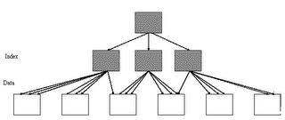
Figure: Good clustering factor

The above image represents "Good CF”. In an event of index range scan, optimizer will not have to jump to next data block as most of the index entries points to same data block. This helps significantly in reducing the cost of your SELECT statements.

Clustering factor is stored in data dictionary and can be viewed from dba_indexes (or user_indexes)

SQL> create table sac as select * from all_objects;

Table created.

SQL> create index obj_id_indx on sac(object_id);

Index created.

SQL> select clustering_factor from user_indexes where index_name='OBJ_ID_INDX';

CLUSTERING_FACTOR
-----------------
545

SQL> select count(*) from sac;

COUNT(*)
----------
38956

SQL> select blocks from user_segments where segment_name='OBJ_ID_INDX';

BLOCKS
----------
96

The above example shows that index has to jump 545 times to give you the full data had you performed full table scan using the index.

Note:
- A good CF is equal (or near) to the values of number of blocks of table.

- A bad CF is equal (or near) to the number of rows of table.

Myth:
- Rebuilding of index can improve the CF.

Then how to improve the CF?

- To improve the CF, it’s the table that must be rebuilt (and reordered).
- If table has multiple indexes, careful consideration needs to be given by which index to order table.



Important point: The above is my interpretation of the subject after reading the book on Optimizer of Jonathan Lewis.

Star Vs Snowflake schema

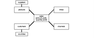
Star Schemas

The star schema is the simplest data warehouse schema. It is called a star schema because the diagram resembles a star, with points radiating from a center. The center of the star consists of one or more fact tables and the points of the star are the dimension tables, as shown in figure.







Fact Tables

A fact table typically has two types of columns: those that contain numeric facts (often called measurements), and those that are foreign keys to dimension tables. A fact table contains either detail-level facts or facts that have been aggregated.


Dimension Tables

A dimension is a structure, often composed of one or more hierarchies, that categorizes data. Dimensional attributes help to describe the dimensional value. They are normally descriptive, textual values.
Dimension tables are generally small in size as compared to fact table.


-To take an example and understand, assume this schema to be of a retail-chain (like wal-mart or carrefour).

Fact will be revenue (money). Now how do you want to see data is called a dimension.



In above figure, you can see the fact is revenue and there are many dimensions to see the same data. You may want to look at revenue based on time (what was the revenue last quarter?), or you may want to look at revenue based on a certain product (what was the revenue for chocolates?) and so on.
In all these cases, the fact is same, however dimension changes as per the requirement.



Note: In an ideal Star schema, all the hierarchies of a dimension are handled within a single table.

Star Query

A star query is a join between a fact table and a number of dimension tables. Each dimension table is joined to the fact table using a primary key to foreign key join, but the dimension tables are not joined to each other. The cost-based optimizer recognizes star queries and generates efficient execution plans for them.






Snoflake Schema

The snowflake schema is a variation of the star schema used in a data warehouse.

The snowflake schema (sometimes callled snowflake join schema) is a more complex schema than the star schema because the tables which describe the dimensions are normalized.







Flips of "snowflaking"



- In a data warehouse, the fact table in which data values (and its associated indexes) are stored, is typically responsible for 90% or more of the storage requirements, so the benefit here is normally insignificant.

- Normalization of the dimension tables ("snowflaking") can impair the performance of a data warehouse. Whereas conventional databases can be tuned to match the regular pattern of usage, such patterns rarely exist in a data warehouse. Snowflaking will increase the time taken to perform a query, and the design goals of many data warehouse projects is to minimize these response times.


Benefits of "snowflaking"



- If a dimension is very sparse (i.e. most of the possible values for the dimension have no data) and/or a dimension has a very long list of attributes which may be used in a query, the dimension table may occupy a significant proportion of the database and snowflaking may be appropriate.



- A multidimensional view is sometimes added to an existing transactional database to aid reporting. In this case, the tables which describe the dimensions will already exist and will typically be normalised. A snowflake schema will hence be easier to implement.

- A snowflake schema can sometimes reflect the way in which users think about data. Users may prefer to generate queries using a star schema in some cases, although this may or may not be reflected in the underlying organisation of the database.

- Some users may wish to submit queries to the database which, using conventional multidimensional reporting tools, cannot be expressed within a simple star schema. This is particularly common in data mining of customer databases, where a common requirement is to locate common factors between customers who bought products meeting complex criteria. Some snowflaking would typically be required to permit simple query tools such as Cognos Powerplay to form such a query, especially if provision for these forms of query weren't anticpated when the data warehouse was first designed.

In practice, many data warehouses will normalize some dimensions and not others, and hence use a combination of snowflake and classic star schema.


Source: Oracle documentation, wikipedia

Touch-Count Algorithm

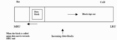
Touch-Count Algorithm:

In advancement to LRU/MRU algorithm, Oracle 8i moves towards an efficient
algorithm of managing the Buffer cache i.e. touch-count algorithm.

Bad SQL design

Important point

If the statement is designed poorly, nothing much can be done by optimizer or indexes

Few known thumb rules

–Avoid Cartesian joins

–Use UNION ALL instead of UNION – if possible

–Use EXIST clause instead of IN - (Wherever appropiate)

–Use order by when you really require it – Its very costly

–When joining 2 views that themselves select from other views, check that the 2 views that you are using do not join the same tables!

–Avoid NOT in or NOT = on indexed columns. They prevent the optimizer from using indexes. Use where amount > 0 instead of where amount != 0


- Avoid writing where is not null. nulls can prevent the optimizer from using an index

- Avoid calculations on indexed columns. Write WHERE amount > 26000/3 instead of WHERE approved_amt/3 > 26000

- The query below will return any record where bmm_code = cORE, Core, CORE, COre, etc.

select appl_appl_id where upper(bmm_code) LIKE 'CORE%'

But this query can be very inefficient as it results in a full table scan. It cannot make use of the index on bmm_code.

Instead, write it like this:

select appl_appl_id from nci_appl_elements_t where (bmm_code like 'C%' or bmm_code like 'c%') and upper(bmm_code) LIKE 'CORE%'

This results in Index Range Scan.

You can also make this more efficient by using 2 characters instead of just one:

where ((bmm_code like 'CO%' or bmm_code like 'Co%' or bmm_code like 'cO%' or bmm_code like 'co%') and upper(bmm_code) LIKE 'CORE%')


Inviting Experts

Friends, feel free to correct me. I will appreciate if you can add your comments also.

Consider declaring NOT NULL columns

Consider declaring NOT NULL columns


People sometimes do not bother to define columns as NOT NULL in the data dictionary, even though these columns should not contain nulls, and indeed never do contain nulls because the application ensures that a value is always supplied. You may think that this is a matter of indifference, but it is not. The optimizer sometimes needs to know that a column is not nullable, and without that knowledge it is constrained to choose a less than optimal execution plan.

1. An index on a nullable column cannot be used to drive access to a table unless the query contains one or more predicates against that column that exclude null values.

Of course, it is not normally desirable to use an index based access path unless the query contains such predicates, but there are important exceptions.

For example, if a full table scan would otherwise be required against the table and the query can be satisfied by a fast full scan (scan for which table data need not be read) against the index, then the latter plan will normally prove more efficient.

Test-case for the above reasoning

SQL> create index color_indx on automobile(color);

Index created.

SQL> select distinct color,count(*) from automobile group by color;


Execution Plan
----------------------------------------------------------
0 SELECT STATEMENT Optimizer=ALL_ROWS (Cost=4 Card=1046 Bytes=
54392)

1 0 SORT (GROUP BY) (Cost=4 Card=1046 Bytes=54392)
2 1 TABLE ACCESS (FULL) OF 'AUTOMOBILE' (TABLE) (Cost=3 Card
=1046 Bytes=54392)


SQL> alter table automobile modify color not null;

Table altered.

SQL> select distinct color,count(*) from automobile group by color;


Execution Plan
----------------------------------------------------------
0 SELECT STATEMENT Optimizer=ALL_ROWS (Cost=4 Card=1046 Bytes=
54392)

1 0 SORT (GROUP BY) (Cost=4 Card=1046 Bytes=54392)
2 1 INDEX (FAST FULL SCAN) OF 'COLOR_INDX' (INDEX) (Cost=3 C
ard=1046 Bytes=54392)



2. If you are calling a sub-query in a parent query using the NOT IN predicate, the indexing on column (in where clause of parent query) will not be used.

Because as per optimizer, results of parent query needs to be displayed only when there is no equi-matching from sub-query, And if the sub-query can potentially contain NULL value (UNKNOWN, incomparable), parent query will have no value to compare with NULL value, so it will not use the INDEX.

Test-case for the above Reasoning

SQL> create index sal_indx on emp(sal);

Index created.

SQL> create index ename_indx on emp(ename);

Index created.

SQL> select * from emp where sal not in (select sal from emp where ename='JONES');


Execution Plan
----------------------------------------------------------
0 SELECT STATEMENT Optimizer=ALL_ROWS (Cost=17 Card=13 Bytes=4
81)

1 0 FILTER
2 1 TABLE ACCESS (FULL) OF 'EMP' (TABLE) (Cost=3 Card=14 Byt
es=518) –> you can see a full table scan even when index exist on SAL

3 1 TABLE ACCESS (BY INDEX ROWID) OF 'EMP' (TABLE) (Cost=2 C
ard=1 Bytes=10)

4 3 INDEX (RANGE SCAN) OF 'ENAME_INDX' (INDEX) (Cost=1 Car
d=1)



SQL> alter table emp modify sal not null;

Table altered.

SQL> select * from emp where sal not in (select sal from emp where ename='JONES');


Execution Plan
----------------------------------------------------------
0 SELECT STATEMENT Optimizer=ALL_ROWS (Cost=5 Card=12 Bytes=56
4)

1 0 MERGE JOIN (ANTI) (Cost=5 Card=12 Bytes=564)
2 1 TABLE ACCESS (BY INDEX ROWID) OF 'EMP' (TABLE) (Cost=2 C
ard=14 Bytes=518)

3 2 INDEX (FULL SCAN) OF 'SAL_INDX' (INDEX) (Cost=1 Card=1
4) -> Here you go, your index getting used now

4 1 SORT (UNIQUE) (Cost=3 Card=1 Bytes=10)
5 4 TABLE ACCESS (BY INDEX ROWID) OF 'EMP' (TABLE) (Cost=2
Card=1 Bytes=10)

6 5 INDEX (RANGE SCAN) OF 'ENAME_INDX' (INDEX) (Cost=1 C
ard=1)


The above article has been an inspiration after reading an article on ixora . The article was missing some of the testcases, so I thought of adding few for newbiews to relate to it.

IN Vs Exist in SQL

IN Vs EXISTS

The two are processed quite differently.


IN Clause

Select * from T1 where x in ( select y from T2 )

is typically processed as:

select *
from t1, ( select distinct y from t2 ) t2
where t1.x = t2.y;

The sub query is evaluated, distinct, indexed and then
joined to the original table -- typically.


As opposed to "EXIST" clause

select * from t1 where exists ( select null from t2 where y = x )

That is processed more like:


for x in ( select * from t1 )
loop
if ( exists ( select null from t2 where y = x.x )
then
OUTPUT THE RECORD
end if
end loop

It always results in a full scan of T1 whereas the first query can make use of
an index on T1(x).


So, when is exists appropriate and in appropriate?

Lets say the result of the subquery
( select y from T2 )

is "huge" and takes a long time. But the table T1 is relatively small and
executing ( select null from t2 where y = x.x ) is fast (nice index on
t2(y)). Then the exists will be faster as the time to full scan T1 and do the
index probe into T2 could be less then the time to simply full scan T2 to build
the subquery we need to distinct on.


Lets say the result of the subquery is small -- then IN is typicaly more
appropriate.


If both the subquery and the outer table are huge -- either might work as well
as the other -- depends on the indexes and other factors.

I wrote this note after searching on same issue and found a simple explanation by Tom Kyte.

Here is the link of original